Band Gap and Band Alignment Prediction of Nitride-Based Semiconductors Using Machine Learning

Band Gap and Band Alignment Prediction of Nitride-Based Semiconductors Using Machine Learning

import pandas as pd
import numpy as np
import matplotlib.pyplot as plt
import seaborn as sns

Reading Data

import camelot
tables = camelot.read_pdf('c8tc05554h1.pdf', pages='3,4,5',
                          flavor="stream",
                          strip_text="\n",
                         row_tol=2) # Similar to Pandas for opening CSV files

# Dynamic naming
varDict=locals()
for i ,table in enumerate(tables):
    varDict['df_'+str(i)]=table.df

df=pd.concat([df_0,df_1,df_2])
df.shape

(301, 32)

df.head()

Feature Correlation Analysis:

The covalent radius, electronegativity, valence, and ionization energy of electrons are most correlated with the band gap.

• R: covalent radius (Å)
• X: electronegativity
• V: valence
• I: first ionization energy (MJ/mole)

18-Feature Dataset

X_18=df.iloc[1:,2:-12].values
X_18.shape

(300, 18)

y_18_off=df.iloc[1:,-2].values
y_18_off.shape

(300,)

y_18_gap=df.iloc[1:,-3].values
y_18_gap.shape

(300,)

Leave-One-Out Cross-Validation (LOOCV)

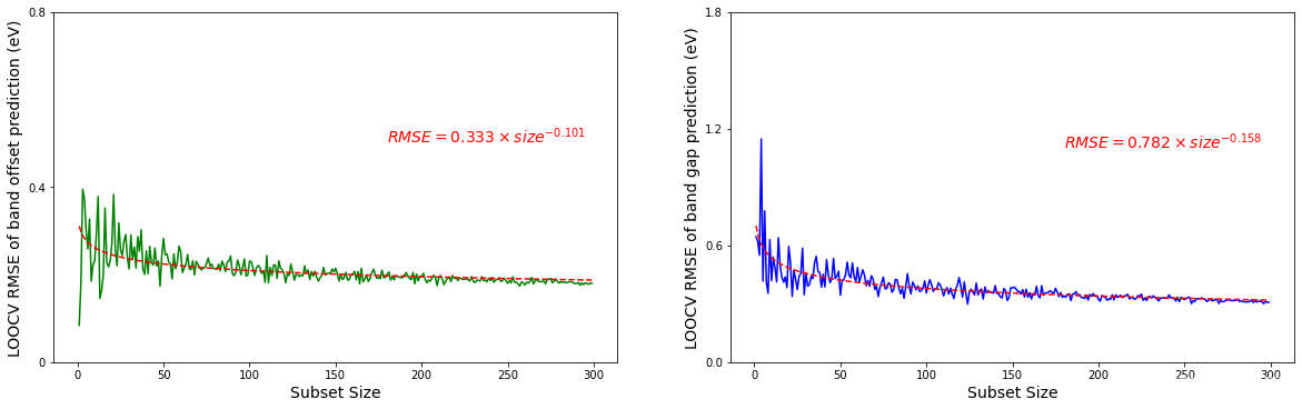
To verify whether the 300 randomly selected nitrides are sufficient to effectively learn the band gap and band offset, we use the RMSE of leave-one-out cross-validation with an SVR model.

from sklearn.model_selection import LeaveOneOut
from sklearn.svm import SVR

# SVR models for predicting band_off and band_gap
svr=SVR(kernel='rbf')

loo=LeaveOneOut()
loo.get_n_splits(X_18)

300

# Function to calculate RMSE
def loocv(X,y,model):
    RMSE=[]
    from sklearn.metrics import mean_squared_error
    for train_index,test_index in loo.split(X):
        X_lo_train,X_lo_test=X[train_index],X[test_index]
        y_lo_train,y_lo_test=y[train_index],y[test_index]
        model.fit(X_lo_train,y_lo_train)
        y_lo_pre=model.predict(X_lo_test)
        rmse=np.sqrt(mean_squared_error(y_lo_test,y_lo_pre)) # Calculate RMSE
        RMSE.append(rmse)


    return RMSE

# Calculate RMSE from leave-one-out for samples 1-299 for band offset
from sklearn.utils import shuffle

rmse_tol_off=[]
for i in range(2,301):
    X_18_sh,y_18_off_sh=shuffle(X_18,y_18_off)
    X_input=X_18_sh[0:i,:]
    y_input=y_18_off_sh[0:i]
    rmse_off=np.mean(np.array(loocv(X_input,y_input,model=svr)))
    rmse_tol_off.append(rmse_off)

# Calculate RMSE from leave-one-out for samples 1-299 for band gap
rmse_tol_gap=[]
for i in range(2,301):
    X_18_sh,y_18_gap_sh=shuffle(X_18,y_18_gap)
    X_input2=X_18_sh[0:i,:]
    y_input2=y_18_gap_sh[0:i]
    rmse_gap=np.mean(np.array(loocv(X_input2,y_input2,model=svr)))
    rmse_tol_gap.append(rmse_gap)

# Define power function
def fun_powder(x,a,b):
    return a*(x**b)

def RMSE_fit(rmse_tol):
    from scipy.optimize import curve_fit
    from sklearn.metrics import mean_squared_error

    ## Fit numerical values and RMSE

    RMSE_fit_curve=[]

    # Calculate optimal parameters a,b
    popt,pcov=curve_fit(fun_powder,np.arange(2,301),np.array(rmse_tol))
    for i in np.arange(2,301):
        rmse_fit=fun_powder(i,popt[0],popt[1])
        RMSE_fit_curve.append(rmse_fit)


    a=popt[0]
    b=popt[1]

    return RMSE_fit_curve,a,b

RMSE_fit_curve_off,a_off,b_off=RMSE_fit(rmse_tol_off)
RMSE_fit_curve_gap,a_gap,b_gap=RMSE_fit(rmse_tol_gap)

fig,ax=plt.subplots(1,2,figsize=(20,5.8))
ax[0].plot(np.arange(1,300),np.array(rmse_tol_off),'g',label='Real curve')
ax[0].plot(np.arange(1,300),RMSE_fit_curve_off,'r--',label='Fitting curve')

ax[1].plot(np.arange(1,300),np.array(rmse_tol_gap),'b',label='Real curve')
ax[1].plot(np.arange(1,300),RMSE_fit_curve_gap,'r--',label='Fitting curve')

ax[0].set_xlabel('Subset Size',fontsize=14)
ax[1].set_xlabel('Subset Size',fontsize=14)

ax[0].set_ylabel('LOOCV RMSE of band offset prediction (eV)',fontsize=14)
ax[1].set_ylabel('LOOCV RMSE of band gap prediction (eV)',fontsize=14)

Figure 1: Leave-one-out cross-validation RMSE as a function of subset size for (left) band offset and (right) band gap prediction. The fitting curves follow power law relationships.

Training Set and Test Set Splitting

# Split into training and test sets
from sklearn.model_selection import train_test_split
X_18_train_off,X_18_test_off,y_18_trian_off,y_18_test_off=train_test_split(X_18,y_18_off,test_size=0.2,
                                                                          random_state=0,shuffle=True)
X_18_train_gap,X_18_test_gap,y_18_trian_gap,y_18_test_gap=train_test_split(X_18,y_18_gap,test_size=0.2,
                                                                          random_state=0,shuffle=True)

Band Offset Regression

SVR Models

# Get training subset and validation subset prediction results
X_18_train_off_sub,X_18_val_off,y_18_trian_off_sub,y_18_val_off=train_test_split(X_18_train_off,
                                                                            y_18_trian_off,test_size=0.25,
                                                                          random_state=0,shuffle=True)

Data Split Strategy:

1. Split dataset into training and test sets with ratio 0.8:0.2
2. Split training set into sub-training set and validation set with ratio 0.75:0.25
3. Final ratio of sub-training:validation:test = 6:2:2

from sklearn.svm import SVR
from sklearn.model_selection import GridSearchCV
from sklearn.model_selection import cross_val_score
svr_linear=SVR(kernel='linear')
svr_poly=SVR(kernel='poly')
svr_rbf=SVR(kernel='rbf')

model_off=[svr_linear,svr_poly,svr_rbf]
param_list_off=[{'C':[25,27,29],'epsilon':[0.01,0.001]},
           {'C':[25,27,29],'epsilon':[0.01,0.001],
                'gamma':[0.1,0.2,0.3],'degree':[6,9,12,15,18]},
           {'C':[25,27,29],'epsilon':[0.01,0.001],
                'gamma':[0.1,0.2,0.3]}]

def final_rmse(model,param,X_train,y_train,X_train_sub,y_train_sub,X_val,y_val):
    """
    X_train,y_train: Total training set
    X_train_sub,y_train_sub: Training subset
    X_val,y_val: Validation set
    """
    gs=GridSearchCV(estimator=model,
                   param_grid=param,
                   cv=10)
    scores=cross_val_score(gs,X_train,y_train,cv=10,
                          scoring='neg_mean_squared_error')
    RMSE=np.sqrt(np.mean(-scores))
    gs.fit(X_train,y_train)
    y_train_pred=gs.best_estimator_.predict(X_train_sub) # Input training subset
    y_val_pred=gs.best_estimator_.predict(X_val)



    return RMSE,y_train_pred,y_val_pred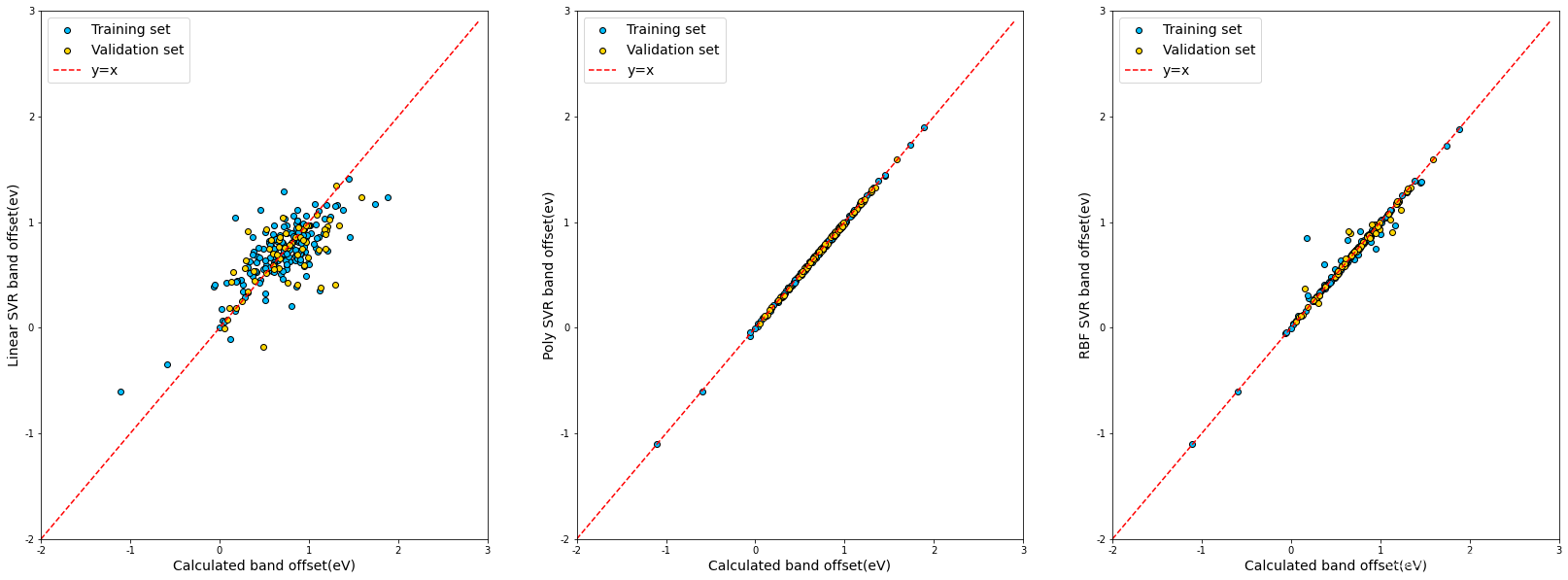

Figure 2: Predicted vs. calculated band offset for Linear, Polynomial, and RBF SVR models. Training set (blue) and validation set (gold) are shown. The RBF kernel achieves the best performance.

Band Gap Regression

18-Features RMSE

The model performance is evaluated using Root Mean Square Error (RMSE) and R² metrics.

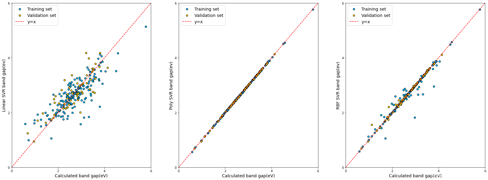
Figure 3: Predicted vs. calculated band gap for Linear, Polynomial, and RBF SVR models using 18 features. The RBF kernel shows superior predictive capability.

19-Features RMSE

Adding PBE (Perdew-Burke-Ernzerhof) feature to improve prediction accuracy.

pbe=df.iloc[1:,-4].values
X_19=np.concatenate((X_18,pbe.reshape(-1,1)),axis=1) # Add PBE feature, making 19 features
X_19.shape

(300, 19)

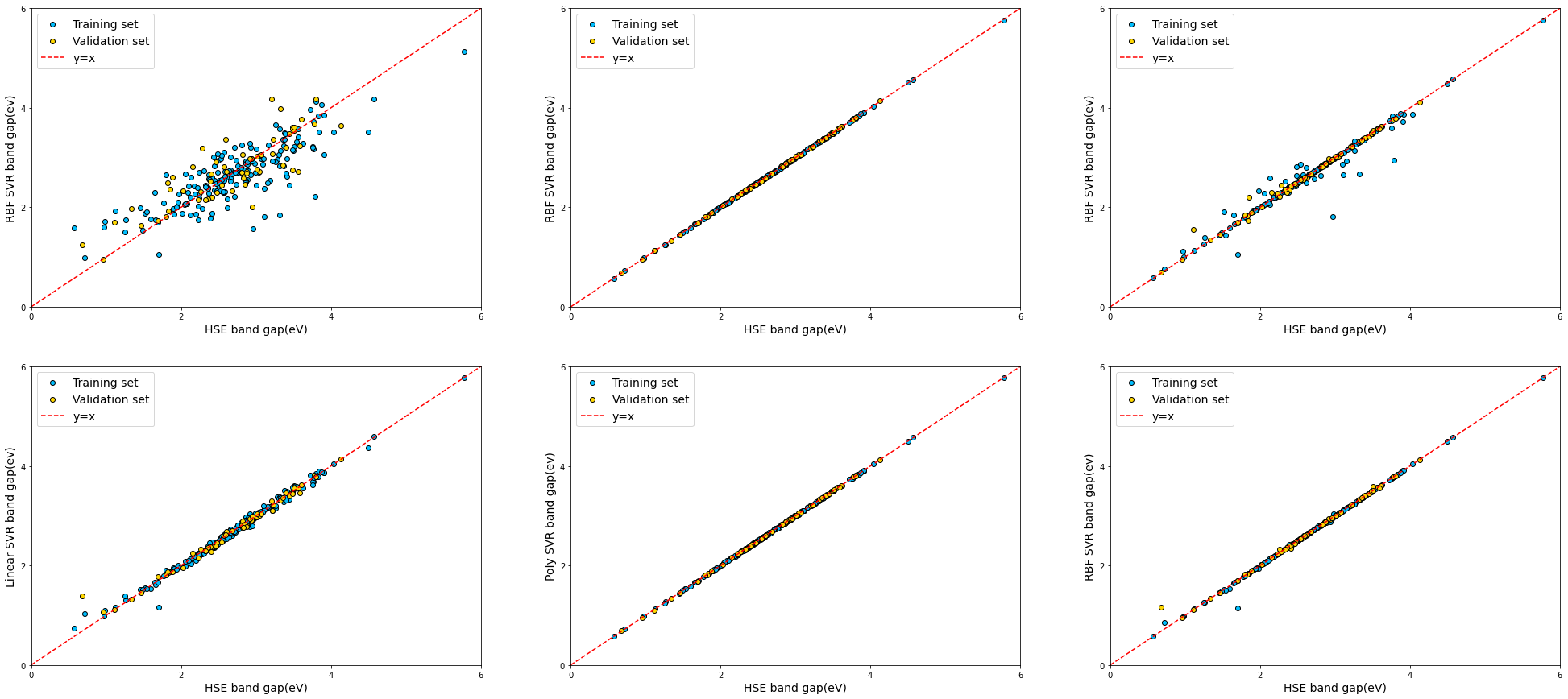
Figure 4: Predicted vs. calculated band gap comparison between 18-feature models (top row) and 19-feature models with added PBE feature (bottom row). The addition of the PBE feature significantly improves prediction accuracy across all three kernel types.

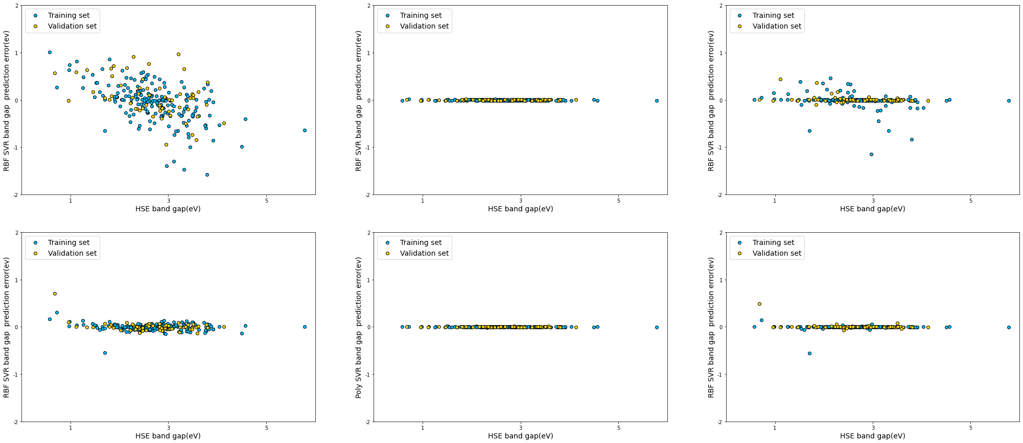
Figure 5: Prediction error distribution showing substantial improvement when PBE feature is included. The 19-feature models (bottom row) show much tighter error distributions centered around zero.

Feature Selection

Using matminer library to convert chemical formulas into pymatgen composition objects and extract features.

from matminer.featurizers.conversions import StrToComposition
data=StrToComposition().featurize_dataframe(df=df,col_id='Nitride')
data.head()

from matminer.featurizers.composition import ElementProperty
ep_feat=ElementProperty.from_preset(preset_name='magpie') # Return ElementProperty from preset string
data=ep_feat.featurize_dataframe(data,'composition') # Convert composition to features
data.head()

Using ElectronegativityDiff feature and guessing oxidation states:

from matminer.featurizers.conversions import CompositionToOxidComposition
from matminer.featurizers.composition import OxidationStates

data=CompositionToOxidComposition().featurize_dataframe(data,'composition')
os_feat=OxidationStates()
data=os_feat.featurize_dataframe(data,'composition_oxid')
data.head()

65,115 Data Histogram Distribution

df_tol=pd.read_excel('半导体.xlsx',sheet_name='Sheet2')

Plot band gap bar distribution and Gaussian fitting

band_gap=df_tol.iloc[:,1]

import seaborn as sns
# Band gap distribution
sns.displot(band_gap,bins=33,color='gold',kde=True)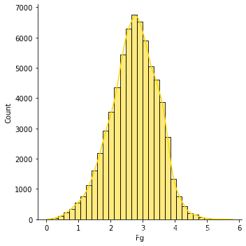

Figure 6: Distribution of band gap values for 67,923 nitride semiconductors with Gaussian kernel density estimation overlay.

band_off=df_tol.iloc[:,1]

# Band offset distribution
sns.displot(band_off,bins=26,color='gray',kde=True)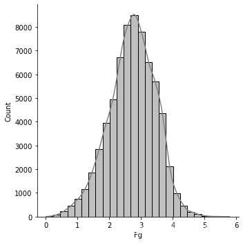

Figure 7: Distribution of band offset values showing the range and frequency of occurrence across the entire dataset.

Summary

This study demonstrates the application of machine learning techniques, specifically Support Vector Regression (SVR) with different kernels (linear, polynomial, RBF), for predicting band gaps and band alignments in nitride-based semiconductors. The results show that:

1. Data Sufficiency: The LOOCV analysis confirms that 300 nitride samples are sufficient for effective learning of band gap and band offset relationships.

1. Feature Importance: Covalent radius, electronegativity, valence, and first ionization energy are the most correlated features with band gap.

1. Model Performance: The RBF-kernel SVR model achieves the best performance among the three kernel types tested.

1. Feature Engineering: Adding the PBE (Perdew-Burke-Ernzerhof) feature improves prediction accuracy, reducing RMSE significantly.

1. Validation: Cross-validation and separate test set evaluation demonstrate good generalization capability of the trained models.

This machine learning approach provides a fast and cost-effective alternative to expensive DFT calculations for initial materials screening and design.