Machine Learning Foundations: Introduction and Linear Regression

This post covers the foundational concepts of machine learning, including supervised and unsupervised learning, with a deep dive into linear regression and gradient descent algorithms.

Introduction to Machine Learning

What is Machine Learning?

Arthur Samuel's Definition (1950s):

Machine learning is the field of study that gives computers the ability to learn without being explicitly programmed.

Tom Mitchell's Formal Definition:

A program is said to learn from experience E with respect to some task T and performance measure P, if its performance on T, as measured by P, improves with experience E.

Example: Spam Email Classification

• Task T: Classify emails as spam or not spam
• Experience E: Observing which emails you mark as spam
• Performance P: Accuracy rate of correct classifications

Types of Machine Learning

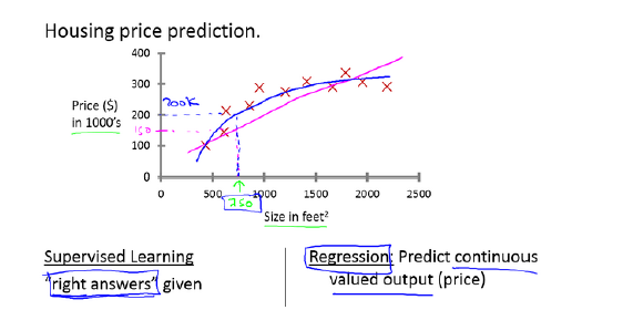
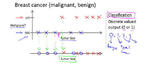
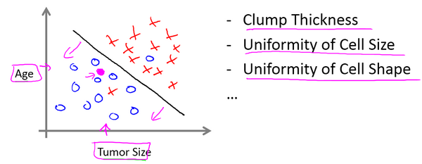
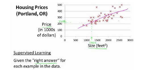
Supervised Learning: Teaching computers with labeled data where "correct answers" are provided

• Regression: Predicting continuous values (e.g., house prices)

• Classification: Predicting discrete categories (e.g., tumor diagnosis)

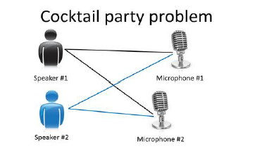
Unsupervised Learning: Finding structure in unlabeled data

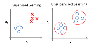
• Clustering: Grouping similar data points
• Applications: Market segmentation, social network analysis, genomics

Linear Regression with One Variable

Model Representation

Housing Price Prediction Example:

• Training set: Historical housing data with prices
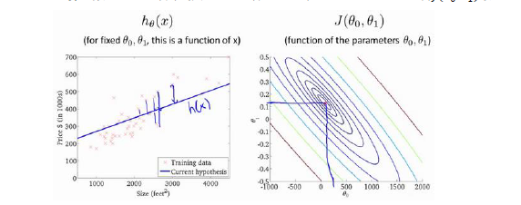
• Goal: Learn a function h(x) that maps house size to predicted price

Notation:

• m: Number of training examples
• x: Input variable/features
• y: Output variable/target
• (x⁽ⁱ⁾, y⁽ⁱ⁾): i-th training example

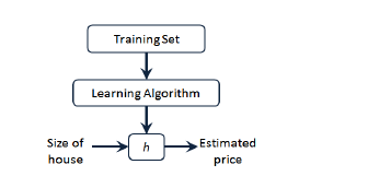
Hypothesis Function:
$h\theta(x) = \theta0 + \theta_1x$

Where θ₀ and θ₁ are the model parameters.

Cost Function

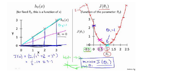
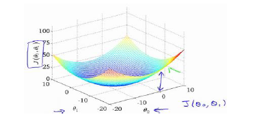
To find optimal parameters, we define a cost function that measures prediction accuracy:

Squared Error Cost Function:
$J(\theta0, \theta1) = \frac{1}{2m} \sum{i=1}^m (h\theta(x^{(i)}) - y^{(i)})^2$

Goal: Find θ₀ and θ₁ that minimize J(θ₀, θ₁)

Gradient Descent

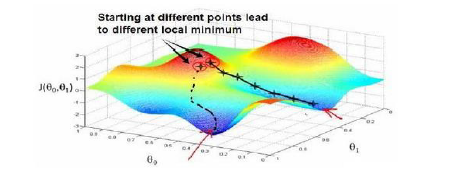
Gradient descent is a general optimization algorithm for finding function minima.

Algorithm:
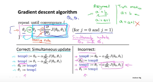
Repeat until convergence {
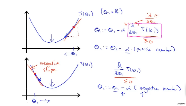
$\thetaj := \thetaj - \alpha \frac{\partial}{\partial\thetaj} J(\theta0, \theta_1)$
}

Where:

• α is the learning rate (controls step size)
• The partial derivative indicates the direction of steepest ascent
• Important: Update θ₀ and θ₁ simultaneously

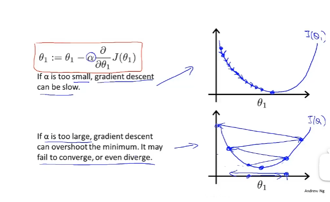
Learning Rate Effects:

• Too small α: Slow convergence
• Too large α: May overshoot and fail to converge

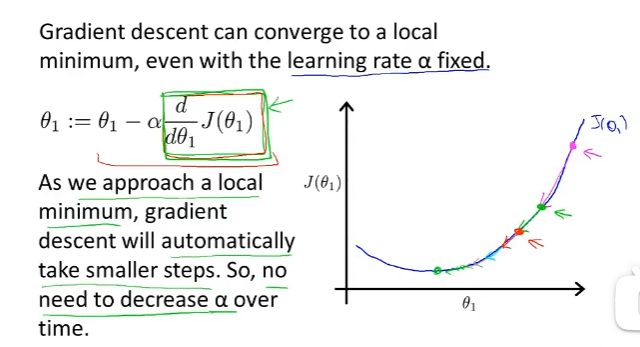
Key Insight: Even with fixed α, gradient descent converges automatically because the gradient decreases as we approach the minimum.

Gradient Descent for Linear Regression

Applying gradient descent to our cost function:

$\theta0 := \theta0 - \alpha \frac{1}{m} \sum{i=1}^{m} (h\theta(x^{(i)}) - y^{(i)})$

$\theta1 := \theta1 - \alpha \frac{1}{m} \sum{i=1}^{m} (h\theta(x^{(i)}) - y^{(i)}) \cdot x^{(i)}$

This is called "Batch" Gradient Descent because each step uses all training examples.

Linear Algebra Review

Matrices and Vectors

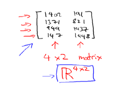
Matrix: Rectangular array of numbers

• Dimension: rows × columns
• Element notation: A_ij (row i, column j)

Vector: Matrix with only one column (n × 1)

• n-dimensional vector
• Indexing: Can use 1-based or 0-based

Matrix Operations

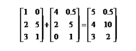
Matrix Addition: Element-wise addition (matrices must have same dimensions)

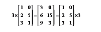
Scalar Multiplication: Multiply each element by the scalar

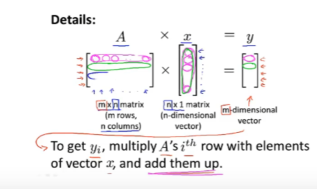
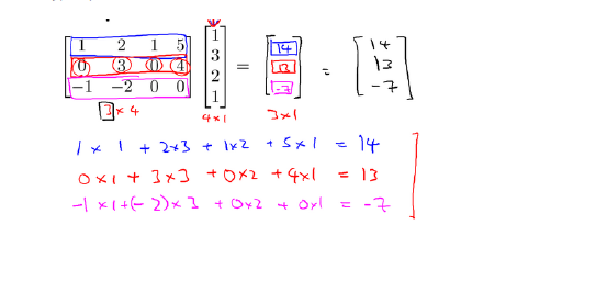
Matrix-Vector Multiplication:

• m × n matrix times n × 1 vector gives m × 1 vector
• Resulti = Rowi · Vector (dot product)

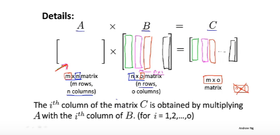
Matrix-Matrix Multiplication:

• m × n matrix times n × o matrix gives m × o matrix
• Resultij = Rowi of A · Column_j of B

Properties:

• Not commutative: A × B ≠ B × A
• Associative: A × (B × C) = (A × B) × C
• Identity matrix I: A × I = I × A = A

Matrix Inverse:

• Only for square matrices
• A × A⁻¹ = A⁻¹ × A = I
• Matrices without inverses are "singular" or "degenerate"

Matrix Transpose:

• (Aᵀ)ij = Aji
• Properties: (A ± B)ᵀ = Aᵀ ± Bᵀ, (A × B)ᵀ = Bᵀ × Aᵀ

Multiple Variable Linear Regression

Multiple Features

Real-world problems often involve multiple features. For house price prediction:

• x₁: Size (sq ft)
• x₂: Number of bedrooms
• x₃: Number of floors
• x₄: Age of home

Notation:

• n: Number of features
• x⁽ⁱ⁾: Feature vector for i-th example
• xⱼ⁽ⁱ⁾: Value of feature j in i-th example

Hypothesis Function:
$h\theta(x) = \theta0 + \theta1x1 + \theta2x2 + ... + \thetanxn$

By convention, define x₀ = 1, then:
$h_\theta(x) = \theta^T x$

Where θ and x are (n+1)-dimensional vectors.

Gradient Descent for Multiple Variables

Cost Function:
$J(\theta) = \frac{1}{2m} \sum{i=1}^{m} (h\theta(x^{(i)}) - y^{(i)})^2$

Update Rule (for j = 0 to n):
$\thetaj := \thetaj - \alpha \frac{1}{m} \sum{i=1}^{m} (h\theta(x^{(i)}) - y^{(i)}) \cdot x_j^{(i)}$

Feature Scaling

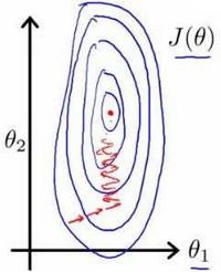
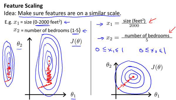
When features have very different ranges, gradient descent converges slowly.

Solution: Mean Normalization
$xn = \frac{xn - \mun}{sn}$

Where:

• μₙ: Mean of feature n
• sₙ: Standard deviation (or max - min)

Goal: Get all features into approximately [-1, 1] range

Learning Rate Selection

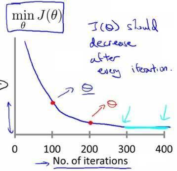
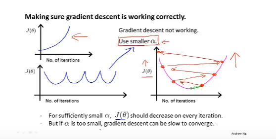
Monitoring Convergence: Plot J(θ) vs. iteration number

• Should decrease after every iteration
• Can use automatic convergence test

Choosing α:

• If J(θ) increases: α is too large
• If convergence is slow: α is too small
• Try values: ..., 0.001, 0.003, 0.01, 0.03, 0.1, 0.3, 1, ...

Polynomial Regression

Sometimes linear models don't fit the data well. We can create polynomial features:

Example:

• Quadratic: $h\theta(x) = \theta0 + \theta1x1 + \theta2x1^2$
• Cubic: $h\theta(x) = \theta0 + \theta1x1 + \theta2x1^2 + \theta3x1^3$
• Square root: $h\theta(x) = \theta0 + \theta1(\text{size}) + \theta2\sqrt{\text{size}}$

Important: Feature scaling becomes crucial with polynomial features!

Normal Equation

Alternative to gradient descent - directly computes optimal θ in one step.

Formula:
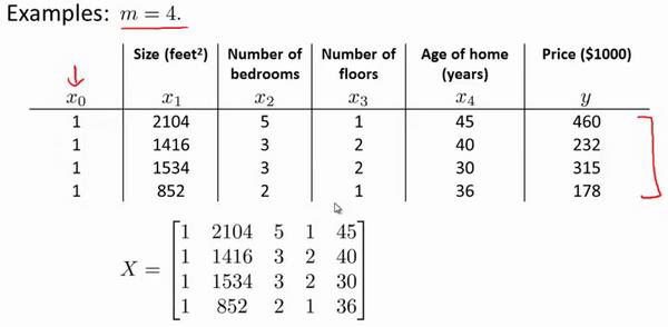
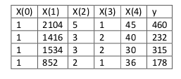
$\theta = (X^T X)^{-1} X^T y$

Where X is the design matrix (m × (n+1)) and y is the target vector (m × 1).

Comparison:

Gradient Descent	Normal Equation
Need to choose α	No need for α
Needs iterations	One-step computation
Works with large n	Slow if n is very large (O(n³))
Works for many models	Only for linear regression

Rule of Thumb: Use normal equation when n < 10,000

Non-Invertibility Issues:
If XᵀX is non-invertible:

1. Check for redundant/linearly dependent features
2. Too many features (n ≥ m): Delete features or use regularization
3. Use pseudoinverse (pinv in software)

---

This completes the foundational material on linear regression and gradient descent. The key takeaways are understanding the hypothesis function, cost function minimization through gradient descent, and the practical considerations of feature scaling and polynomial features.