Machine Learning Logistic Regression and Regularization
· (updated ) · Machine Learning · 6 minute read
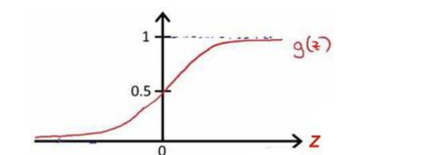
Logistic regression and regularization: decision boundaries, the sigmoid cost function, and L1/L2 penalties to prevent overfitting.
This post explores classification problems through logistic regression and introduces regularization techniques to prevent overfitting.
Classification and Logistic Regression
Classification Problems
Unlike regression (predicting continuous values), classification predicts discrete categories.
Binary Classification: Output y ∈ {0, 1}
- 0: Negative class
- 1: Positive class
Examples:
- Email: Spam (1) or Not Spam (0)
- Tumor: Malignant (1) or Benign (0)
- Transaction: Fraudulent (1) or Legitimate (0)
Why Linear Regression Fails for Classification:
- Predictions can be >> 1 or << 0
- Threshold at 0.5 breaks with outliers
- Not a natural fit for discrete outputs
Hypothesis Representation
Logistic Function (Sigmoid Function):
$g(z) = \frac{1}{1 + e^{-z}}$
Properties:
- Range: (0, 1)
- g(0) = 0.5
- As z → ∞, g(z) → 1
- As z → -∞, g(z) → 0

Logistic Regression Hypothesis:
$h_\theta(x) = g(\theta^T x) = \frac{1}{1 + e^{-\theta^T x}}$
Interpretation: h_θ(x) = Probability that y = 1 given x, parameterized by θ
$h_\theta(x) = P(y=1 | x; \theta)$
Example: If h_θ(x) = 0.7 for a tumor, there's a 70% probability it's malignant.
Decision Boundary
Prediction Rule:
- Predict y = 1 if h_θ(x) ≥ 0.5 (equivalently, θᵀx ≥ 0)
- Predict y = 0 if h_θ(x) < 0.5 (equivalently, θᵀx < 0)
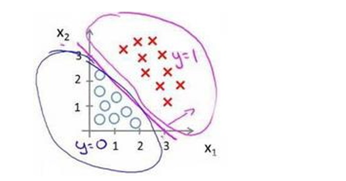
Decision Boundary: The line/surface where θᵀx = 0
Linear Decision Boundary Example:
If h_θ(x) = g(θ₀ + θ₁x₁ + θ₂x₂) with θ = [-3, 1, 1]ᵀ
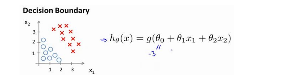
Decision boundary: x₁ + x₂ = 3 (a straight line)
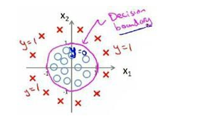
Non-linear Decision Boundary:
With polynomial features: h_θ(x) = g(θ₀ + θ₁x₁ + θ₂x₂ + θ₃x₁² + θ₄x₂²)
If θ = [-1, 0, 0, 1, 1]ᵀ, decision boundary: x₁² + x₂² = 1 (a circle)
Cost Function
Why not use squared error?
The squared error cost function with logistic hypothesis is non-convex, leading to many local minima.
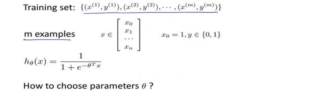
Logistic Regression Cost Function:
$Cost(h_\theta(x), y) = \begin{cases}
-\log(h_\theta(x)) & \text{if } y = 1 \\
-\log(1 - h_\theta(x)) & \text{if } y = 0
\end{cases}$
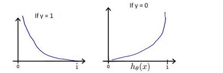
Properties:
- When y = 1:
- Cost → 0 as h_θ(x) → 1 (correct prediction)
- Cost → ∞ as h_θ(x) → 0 (very wrong prediction)
- When y = 0:
- Cost → 0 as h_θ(x) → 0 (correct prediction)
- Cost → ∞ as h_θ(x) → 1 (very wrong prediction)
Simplified Cost Function:
$J(\theta) = -\frac{1}{m} \sum{i=1}^{m} [y^{(i)} \log(h\theta(x^{(i)})) + (1-y^{(i)}) \log(1 - h_\theta(x^{(i)}))]$
This is convex and can be minimized using gradient descent.
Gradient Descent
Update Rule (remarkably similar to linear regression!):
$\thetaj := \thetaj - \alpha \frac{1}{m} \sum{i=1}^{m} (h\theta(x^{(i)}) - y^{(i)}) x_j^{(i)}$
Key Difference: h_θ(x) = sigmoid(θᵀx), not θᵀx
Feature scaling is equally important for logistic regression.
Advanced Optimization
Beyond gradient descent, more sophisticated algorithms exist:
- Conjugate Gradient
- BFGS
- L-BFGS
Advantages:
- No need to manually choose learning rate α
- Often faster convergence
Disadvantage:
- More complex implementation
Recommendation: Use well-tested libraries (e.g., fminunc in Octave, scipy.optimize in Python)
Multiclass Classification: One-vs-All
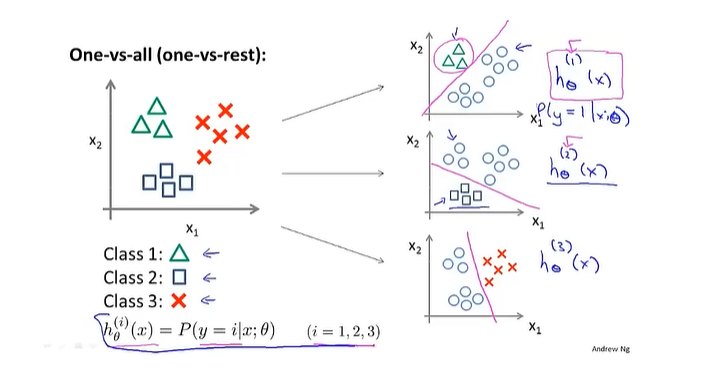
Problem: Classify into K > 2 classes (e.g., email categories: work, friends, family)
Solution: Train K separate binary classifiers
One-vs-All Strategy:
- For each class i:
- Create a binary classification problem: class i (y=1) vs. all others (y=0)
- Train classifier h_θ⁽ⁱ⁾(x)
- For a new example x:
- Run all K classifiers
- Pick the class i with highest h_θ⁽ⁱ⁾(x)
$\text{prediction} = \maxi h\theta^{(i)}(x)$
Regularization
The Problem of Overfitting
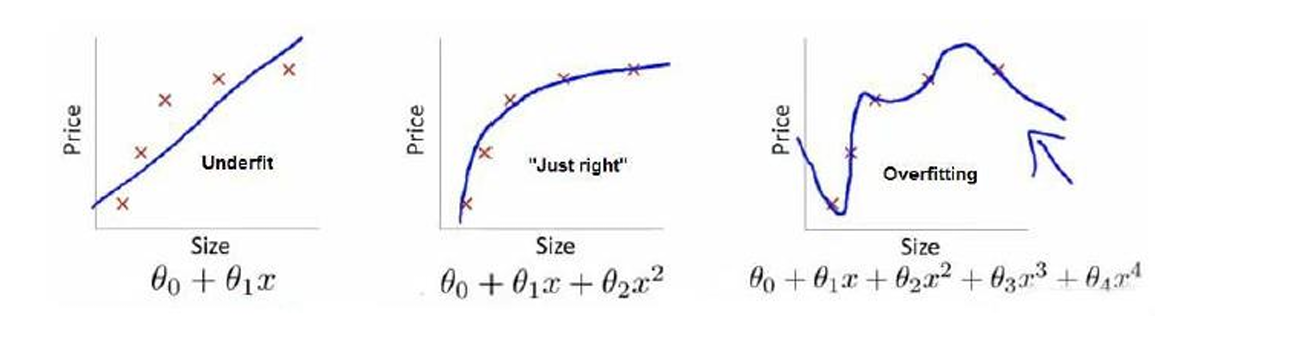
Underfitting (High Bias): Model is too simple, fails to capture data patterns
Overfitting (High Variance): Model is too complex, fits training data perfectly but fails to generalize
Example - Polynomial Regression:
- Linear (underfit): Misses the curve
- Quadratic (just right): Fits well
- High-degree polynomial (overfit): Passes through all points but wiggles unreasonably
Addressing Overfitting:
- Reduce number of features
- Manually select features to keep
- Use model selection algorithms
- Drawback: May discard useful information
- Regularization
- Keep all features but penalize large parameter values
- Works well when many features contribute slightly to prediction
Regularized Cost Function
Intuition: Large parameter values lead to overly complex models. Penalize them!
Regularized Linear Regression:
$J(\theta) = \frac{1}{2m} \left[ \sum{i=1}^{m} (h\theta(x^{(i)}) - y^{(i)})^2 + \lambda \sum{j=1}^{n} \thetaj^2 \right]$
Where:
- λ: Regularization parameter
- λ too large → Underfitting (all θⱼ ≈ 0)
- λ too small → Overfitting
- By convention, don't regularize θ₀
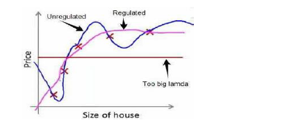
Regularized Linear Regression
Gradient Descent Update:
For θ₀:
$\theta0 := \theta0 - \alpha \frac{1}{m} \sum{i=1}^{m} (h\theta(x^{(i)}) - y^{(i)}) x_0^{(i)}$
For θⱼ (j ≥ 1):
$\thetaj := \thetaj - \alpha \left[ \frac{1}{m} \sum{i=1}^{m} (h\theta(x^{(i)}) - y^{(i)}) xj^{(i)} + \frac{\lambda}{m} \thetaj \right]$
Equivalently:
$\thetaj := \thetaj(1 - \alpha\frac{\lambda}{m}) - \alpha \frac{1}{m} \sum{i=1}^{m} (h\theta(x^{(i)}) - y^{(i)}) x_j^{(i)}$
The factor (1 - α λ/m) < 1 shrinks θⱼ on each iteration.
Normal Equation:
$\theta = (X^T X + \lambda L)^{-1} X^T y$
Where L is an (n+1) × (n+1) matrix with 0 in top-left and 1s on the rest of diagonal.
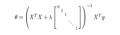
Benefit: This formula is always invertible when λ > 0!
Regularized Logistic Regression
Cost Function:
$J(\theta) = -\frac{1}{m} \sum{i=1}^{m} [y^{(i)} \log(h\theta(x^{(i)})) + (1-y^{(i)}) \log(1 - h\theta(x^{(i)}))] + \frac{\lambda}{2m} \sum{j=1}^{n} \theta_j^2$
Gradient Descent:
Form is identical to regularized linear regression:
For θ₀:
$\theta0 := \theta0 - \alpha \frac{1}{m} \sum{i=1}^{m} (h\theta(x^{(i)}) - y^{(i)}) x_0^{(i)}$
For θⱼ (j ≥ 1):
$\thetaj := \thetaj - \alpha \left[ \frac{1}{m} \sum{i=1}^{m} (h\theta(x^{(i)}) - y^{(i)}) xj^{(i)} + \frac{\lambda}{m} \thetaj \right]$
Remember: h_θ(x) = sigmoid(θᵀx) for logistic regression!
Key Takeaways
- Logistic Regression is the go-to algorithm for binary classification
- The sigmoid function maps any real number to (0,1), providing probability estimates
- Decision boundaries can be linear or non-linear (with polynomial features)
- Regularization prevents overfitting by penalizing large parameter values
- The regularization parameter λ controls the bias-variance tradeoff
- Advanced optimization algorithms can significantly speed up training
Understanding these concepts provides a solid foundation for tackling classification problems in machine learning applications.