Machine Learning Neural Networks

This post explores neural networks, from their biological inspiration to practical implementation of learning algorithms including backpropagation.

Neural Networks: Representation

Why Neural Networks?

The Challenge of Non-linear Hypotheses

For complex non-linear problems, traditional methods face computational limitations:

• With 100 features, quadratic terms alone create ~5,000 new features
• For cubic terms, this explodes even further
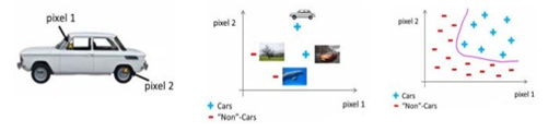
• Example: 50×50 pixel grayscale image = 2,500 features

• All quadratic terms ≈ 3 million features!

Computer Vision Challenge: Recognizing cars in images requires handling massive feature spaces efficiently.

Inspiration: The Brain

"One Learning Algorithm" Hypothesis

Remarkable neuroscience experiments suggest the brain uses a single learning algorithm:

• Neural Rewiring: Auditory cortex can learn to "see" when connected to optical nerves
• Somatosensory cortex can learn to "see"
• The brain shows remarkable plasticity

Modern Applications:

• BrainPort: Camera on forehead → electrode array on tongue → blind people learn to "see"

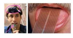
• Human Echolocation: Blind individuals use tongue clicks to navigate like bats
• Haptic Belt: Always points north → users develop direction sense

Insight: If we can discover and implement the brain's learning algorithm, we may unlock true AI.

Artificial Neural Network Model

Neuron:

• Inputs: Dendrites receive signals
• Processing: Cell body (soma) computes
• Output: Axon transmits signals (spikes)

Artificial Neuron (Logistic Unit):

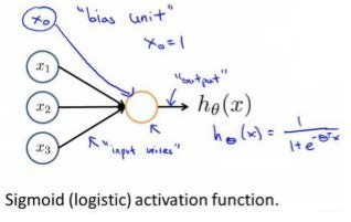
Inputs: x₁, x₂, x₃
Bias: x₀ = 1
Parameters: θ (weights)
Activation function: g(z) = sigmoid(θᵀx)
Output: h_θ(x)

Neural Network Architecture:

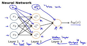
• Layer 1 (Input): Raw features [x₀, x₁, x₂, x₃]
• Layer 2 (Hidden): Computed features [a₀⁽²⁾, a₁⁽²⁾, a₂⁽²⁾, a₃⁽²⁾]
• Layer 3 (Output): Final prediction h_θ(x)

Notation:

• aᵢ⁽ʲ⁾: Activation of unit i in layer j
• Θ⁽ʲ⁾: Matrix of weights mapping from layer j to j+1
• If layer j has sⱼ units and layer j+1 has sⱼ₊₁ units, Θ⁽ʲ⁾ is sⱼ₊₁ × (sⱼ + 1)

Forward Propagation

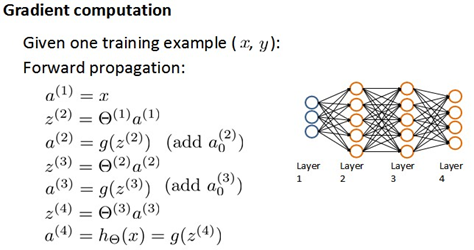
Vectorized Computation:

Layer 2 activations:

z⁽²⁾ = Θ⁽¹⁾x
a⁽²⁾ = g(z⁽²⁾)
Add a₀⁽²⁾ = 1

Layer 3 (output):

z⁽³⁾ = Θ⁽²⁾a⁽²⁾
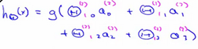
h_θ(x) = a⁽³⁾ = g(z⁽³⁾)

Key Insight: Neural networks learn their own features!

• Hidden layer activations a⁽²⁾ are "learned features"

• More powerful than hand-crafted polynomial features
• The network automatically discovers useful feature representations

Neural Networks for Logic Functions

AND Function:

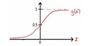
Θ⁽¹⁾ = [-30, 20, 20]
h_θ(x) = g(-30 + 20x₁ + 20x₂)

Truth table:

• (0,0) → 0, (0,1) → 0, (1,0) → 0, (1,1) → 1 ✓

OR Function:

Θ⁽¹⁾ = [-10, 20, 20]

NOT Function:

Θ = [10, -20]
h_θ(x₁) = g(10 - 20x₁)

XNOR (Complex Function):

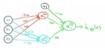
Combine simpler functions in layers:

• Layer 1: (x₁ AND x₂), (NOT x₁ AND NOT x₂)
• Layer 2: OR of layer 1 outputs

This demonstrates how neural networks can learn arbitrarily complex functions through composition!

Multiclass Classification

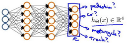
One-vs-All Extended:
For K classes, output layer has K units using one-hot encoding:

Example: 4-class classification

Pedestrian:  [1, 0, 0, 0]ᵀ
Car:         [0, 1, 0, 0]ᵀ
Motorcycle:  [0, 0, 1, 0]ᵀ
Truck:       [0, 0, 0, 1]ᵀ

The network outputs a K-dimensional vector where h_θ(x)ᵢ ≈ P(y = i | x; θ)

Neural Networks: Learning

Cost Function

Notation:

• L: Total number of layers
• sₗ: Number of units in layer l
• K: Number of output units (classes)

Binary Classification (K=1):

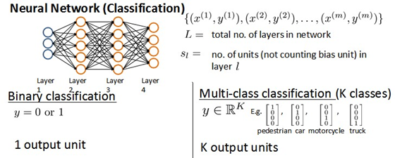
• Output layer has 1 unit
• y ∈ {0, 1}

Multi-class Classification (K≥3):

• Output layer has K units
• y ∈ ℝᴷ (one-hot vector)

Neural Network Cost Function:

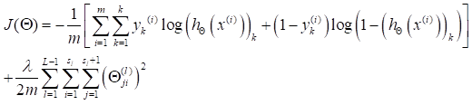
$J(\Theta) = -\frac{1}{m} \sum{i=1}^{m} \sum{k=1}^{K} [yk^{(i)} \log(h\Theta(x^{(i)}))k + (1-yk^{(i)}) \log(1-(h\Theta(x^{(i)}))k)]$
$+ \frac{\lambda}{2m} \sum{l=1}^{L-1} \sum{i=1}^{sl} \sum{j=1}^{s{l+1}} (\Theta{ji}^{(l)})^2$

This is a generalization of logistic regression cost:

• Sum over all K output units
• Sum over all m training examples
• Regularization term sums over all network weights (excluding bias terms)

Backpropagation Algorithm

The Challenge: Computing ∂J/∂Θᵢⱼ⁽ˡ⁾ efficiently

Intuition: "Error propagation" from output to input

• δ⁽ˡ⁾: "Error" of layer l nodes
• Represents how much each node is "responsible" for final errors

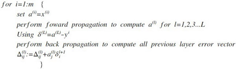
Algorithm (for single training example):

1. Forward pass: Compute all activations

   a⁽¹⁾ = x
   z⁽ˡ⁺¹⁾ = Θ⁽ˡ⁾a⁽ˡ⁾
   a⁽ˡ⁺¹⁾ = g(z⁽ˡ⁺¹⁾)

1. Compute output error:

   δ⁽ᴸ⁾ = a⁽ᴸ⁾ - y

1. Backpropagate error:

   δ⁽ˡ⁾ = (Θ⁽ˡ⁾)ᵀ δ⁽ˡ⁺¹⁾ .* g'(z⁽ˡ⁾)

where g'(z⁽ˡ⁾) = a⁽ˡ⁾ .* (1 - a⁽ˡ⁾)

1. Compute gradients:

   ∂J/∂Θᵢⱼ⁽ˡ⁾ = aⱼ⁽ˡ⁾ δᵢ⁽ˡ⁺¹⁾

For entire training set:

Initialize: Δ⁽ˡ⁾ = 0 (for all l)

for i = 1 to m:
    # Forward propagation

![Forward Propagation](/images/blog/2023-07-15-ml-week5-6-neural-networks/forward-propagation.png)

    Compute a⁽ˡ⁾ for all layers

    # Backward propagation
    Compute δ⁽ˡ⁾ for all layers

    # Accumulate gradients
    Δ⁽ˡ⁾ := Δ⁽ˡ⁾ + δ⁽ˡ⁺¹⁾(a⁽ˡ⁾)ᵀ

# Compute final gradients
Dᵢⱼ⁽ˡ⁾ = (1/m)Δᵢⱼ⁽ˡ⁾ + (λ/m)Θᵢⱼ⁽ˡ⁾    (if j ≠ 0)
Dᵢⱼ⁽ˡ⁾ = (1/m)Δᵢⱼ⁽ˡ⁾                  (if j = 0)

Gradient Checking

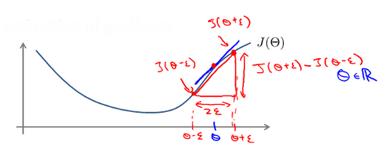
Purpose: Verify backpropagation implementation is correct

Numerical Gradient Approximation:
$\frac{\partial J}{\partial \theta} \approx \frac{J(\theta + \epsilon) - J(\theta - \epsilon)}{2\epsilon}$

where ε ≈ 10⁻⁴

Implementation:

for i in range(len(theta)):
    theta_plus = theta.copy()
    theta_minus = theta.copy()
    theta_plus[i] += epsilon
    theta_minus[i] -= epsilon
    gradApprox[i] = (J(theta_plus) - J(theta_minus)) / (2*epsilon)

# Check: gradApprox ≈ gradient_from_backprop

CRITICAL: Disable gradient checking during training (very slow!)

Random Initialization

Why not initialize to zero?

• All hidden units would compute identical functions
• Symmetric breaking problem
• Network would fail to learn diverse features

Solution: Initialize randomly in [-ε, ε]

epsilon_init = 0.12
Theta = np.random.rand(L_out, L_in + 1) * 2 * epsilon_init - epsilon_init

Complete Training Pipeline

1. Choose Architecture:

• Input units = number of features
• Output units = number of classes
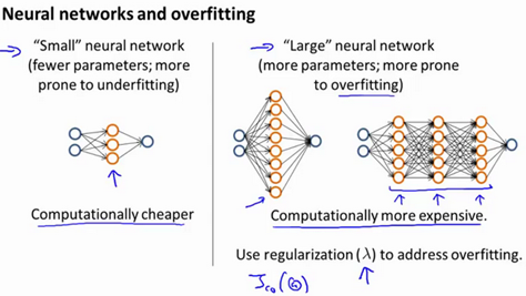
• Hidden layers: More is usually better (use regularization to prevent overfitting)
• Units per hidden layer: Often same across all hidden layers

1. Training:

   # Random initialization
   Initialize Θ randomly

   # Optimize using advanced method
   for iteration in range(num_iterations):
       # Forward propagation
       for each example: compute h_Θ(x)

       # Compute cost J(Θ)

       # Backpropagation
       for each example: compute gradients

       # Update parameters (using gradient descent or advanced optimizer)

1. Gradient Checking (during debugging only)

1. Use optimization algorithm with backpropagation to minimize J(Θ)

Example: ALVINN (Autonomous Driving)

Historic Application (1989):

• Input: 30×32 pixel road image
• Network: 3 layers
• Output: Steering direction
• Trained by observing human drivers

Multiple Networks:

• Separate networks for different road types
• System selects most confident network
• Smooth transitions between networks

This demonstrated neural networks could master complex real-world tasks with sufficient training data!

---

Key Takeaways

1. Neural networks learn hierarchical feature representations automatically
2. Backpropagation efficiently computes gradients through chain rule
3. Gradient checking is essential for debugging but must be disabled during training
4. Random initialization breaks symmetry and enables learning
5. Architecture choices significantly impact performance:

• More hidden units/layers = more capacity
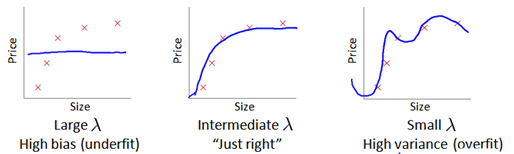
• Regularization prevents overfitting

1. Even relatively simple networks can solve complex problems (e.g., autonomous driving)

Understanding these fundamentals provides a solid foundation for modern deep learning!