Machine Learning-Aided Design of Aluminum Alloys

Machine Learning-Aided Design of Aluminum Alloys

Al-Cu-Mg-x alloys were selected as the base material for this study.

import numpy as np
import pandas as pd
import seaborn as sns
import matplotlib.pyplot as plt

data=pd.read_excel('1-s2.0-S2352492820329081-mmc1.xlsx',header=1)
data.head()

data.dropna(axis=1,inplace=True)
data.head()

Dataset Description

Features of various Al-Cu-Mg-x based alloys including composition, aging conditions (temperature and time), and related properties (hardness).

Physical Properties $X_{i}$: Electronegativity, atomic number, atomic mass, atomic radius, valence electrons, boiling point, specific heat, melting point, heat of vaporization, heat of fusion, group, period, electron affinity, density, thermal conductivity of element i.

Concentration $C_{i}$: Concentration of element i in the alloy

Feature Weighted Fraction: $X=\Sigma C{i} X{i}$

where X is the weighted fractional feature.

data.info()

<class 'pandas.core.frame.DataFrame'>
RangeIndex: 1591 entries, 0 to 1590
Data columns (total 34 columns):

Column Non-Null Count Dtype

--- ------ -------------- -----
0 Hardness 1591 non-null int64
1 Al 1591 non-null float64
2 Cu 1591 non-null float64
3 Mg 1591 non-null float64
...

LOF Anomaly Detection

Local Outlier Factor (LOF) is used to identify anomalies in the dataset. Each sample's anomaly level is called the local outlier factor. It measures the local density deviation of a given sample relative to its neighbors. The locality is determined by k-nearest neighbors, whose distances are used to estimate local density. By comparing a sample's local density with its neighbors' densities, we can identify samples with significantly lower density than their neighbors as outliers.

Parameters:

• n_neighbors: If n_neighbors is greater than the provided number of samples, all samples will be used
• algorithm: {'auto', 'balltree', 'kdtree', 'brute'}

df=data.values
df.shape

(1591, 34)

from sklearn.neighbors import LocalOutlierFactor

# Group of 10 samples, outlier ratio is 0.055 (similar to the paper)
LOF=LocalOutlierFactor(n_neighbors=10,contamination=0.055)
# Inliers marked as 1, outliers as -1
labels=LOF.fit_predict(df)
# Data after LOF verification
df=df[labels>0]
df.shape

(1503, 34)

y=df[:,0]
y.shape

(1503,)

X=df[:,1:]
X.shape

(1503, 33)

Data Splitting and Standardization

from sklearn.model_selection import train_test_split
X_train,X_test,y_train,y_test=train_test_split(X,
                                               y,
                                               test_size=0.4,
                                               random_state=0)

X_train.shape,X_test.shape

((901, 33), (602, 33))

from sklearn.preprocessing import StandardScaler
sc1=StandardScaler()
X_train=sc1.fit_transform(X_train)
X_test=sc1.transform(X_test)
sc2=StandardScaler()
y_train=sc2.fit_transform(y_train.reshape(-1,1))
y_test=sc2.transform(y_test.reshape(-1,1))
y_test_inverse=sc2.inverse_transform(y_test) # Inverse normalization

Feature Selection

Filter Method

name_list=list(data.columns[17:]) # Modify original list
name_list.append('Hardness')
name=pd.Index(name_list)
name_list

['EN',
'VE',
'Atomic number',
'mass',
'Melting point',
'Boiling point',
'Density',
'Electroaffinity',
'Fusion heat',
'atomic radius',
'Specfic heat',
'Heat of Vaporization',
'thermal conductivity',
'group',
'period',
'Time (min)',
'Temperature (K)',
'Hardness']

name_del=data.columns[1:17]

corr_data=np.concatenate((np.delete(X,axis=1,obj=np.arange(0,16)),y.reshape(-1,1)),
                         axis=1)
corr_data.shape

(1503, 18)

# Using filter correlation coefficient method

corr_df=pd.DataFrame(corr_data,columns=name)

corr_df=corr_df.corr()
# Plot heatmap
plt.figure(figsize=(15,15))
sns.heatmap(corr_df,vmax=1.0,vmin=-1.0,
           cmap='rainbow',
           xticklabels=name_list,
            yticklabels=name_list,annot=True,fmt=".2f")

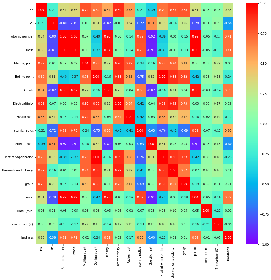
Figure 1: Correlation matrix heatmap showing relationships between features and hardness. Features with |r| < 0.45 are considered uncorrelated and will be removed.

# Determine features to delete
fil_features=corr_df.index[abs(corr_df['Hardness'])<0.45]
fil_features

Index(['EN', 'Melting point', 'Boiling point', 'Electroaffinity',
'Fusion heat', 'Heat of Vaporization', 'thermal conductivity', 'group',
'Time (min)', 'Temperature (K)'],
dtype='object')

Correlation Analysis: Features with correlation coefficient r between -0.45 and 0.45 are considered uncorrelated.

WFS (Wrapper Feature Selection)

from sklearn.feature_selection import RFE
from sklearn.svm import SVR

# Build RFE
estimator = SVR(kernel="linear")
selector = RFE(estimator, n_features_to_select=14, step=1)
selector.fit(np.delete(X,axis=1,obj=np.arange(0,16)),y)

# Get deleted features
name_wfs_list=list(data.columns[17:])
name_wfs=pd.Index(name_wfs_list)

name_wfs[~selector.support_]

Index(['thermal conductivity', 'Time (min)', 'Temperature (K)'], dtype='object')

Note: 'Time (min)' and 'Temperature (K)' have significant relationship with hardness.

Model Training

Comparing performance of:

• General Linear Models (GLM)
• Deep Learning (DL)
• Decision Tree (DT)
• Random Forest (RF)
• Gradient Boosting Tree (GBT)
• Support Vector Machine (SVM)

Performance metrics:

• Mean Squared Error (MSE): $MSE=1/n \Sigma{i=1}^{n}(yi-\hat y_i)^{2}$
• R² statistic

Without Optimization

# SVR
from sklearn.svm import SVR
svr=SVR()
svr.fit(X_train,y_train.ravel())
y_svr_pred=svr.predict(X_test)

# GBT (Gradient Boosting Tree)
from sklearn.ensemble import GradientBoostingRegressor
gbt=GradientBoostingRegressor(random_state=0)
gbt.fit(X_train,y_train.ravel())
y_gbt_pred=gbt.predict(X_test)

# RF (Random Forest)
from sklearn.ensemble import RandomForestRegressor
rf=RandomForestRegressor(random_state=0)
rf.fit(X_train,y_train.ravel())
y_rf_pred=rf.predict(X_test)

# Decision Tree
from sklearn.tree import DecisionTreeRegressor
dt=DecisionTreeRegressor(random_state=0)
dt.fit(X_train,y_train.ravel())
y_dt_pred=dt.predict(X_test)

# MLP Regressor
from sklearn.neural_network import MLPRegressor
mlp=MLPRegressor(random_state=0,max_iter=800)
mlp.fit(X_train,y_train.ravel())
y_mlp_pred=mlp.predict(X_test)

# Ridge Regression
from sklearn.linear_model import Ridge
ridge=Ridge(random_state=0)
ridge.fit(X_train,y_train.ravel())
y_ridge_pred=ridge.predict(X_test)

def compute_r2(y_true,y_pred):
    from sklearn.metrics import r2_score
    r2=r2_score(y_true,y_pred)
    return r2

def compute_mse(y_true,y_pred):
    from sklearn.metrics import mean_squared_error
    mse=mean_squared_error(y_true,y_pred)
    return mse

# Calculate on test set
y_pred_list=[y_svr_pred,y_gbt_pred,y_rf_pred,
       y_dt_pred,y_mlp_pred,y_ridge_pred]
r2_list=[]
mse_list=[]
for i in np.arange(0,6):
    r2=compute_r2(y_test,y_pred_list[i])
    r2_list.append(r2)
    mse=compute_mse(y_test,y_pred_list[i])
    mse_list.append(mse)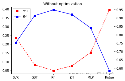

Figure 2: Comparison of MSE and R² scores for six different regression models without hyperparameter optimization. Random Forest and Gradient Boosting show promising results.

# 5-fold cross-validation RMSE
def cross_val_MSE(model,X,y,test_size=0.25):
    from sklearn.model_selection import cross_val_score,ShuffleSplit
    scores_model=cross_val_score(estimator=model,
                                 X=X,
                                 y=y,
                                 cv=ShuffleSplit(n_splits=100,test_size=test_size),
                                scoring='neg_mean_squared_error') # ShuffleSplit shuffles data
    return np.mean(-scores_model)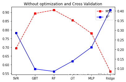

Figure 3: Cross-validation results showing model performance with shuffled data splits, providing more robust evaluation.

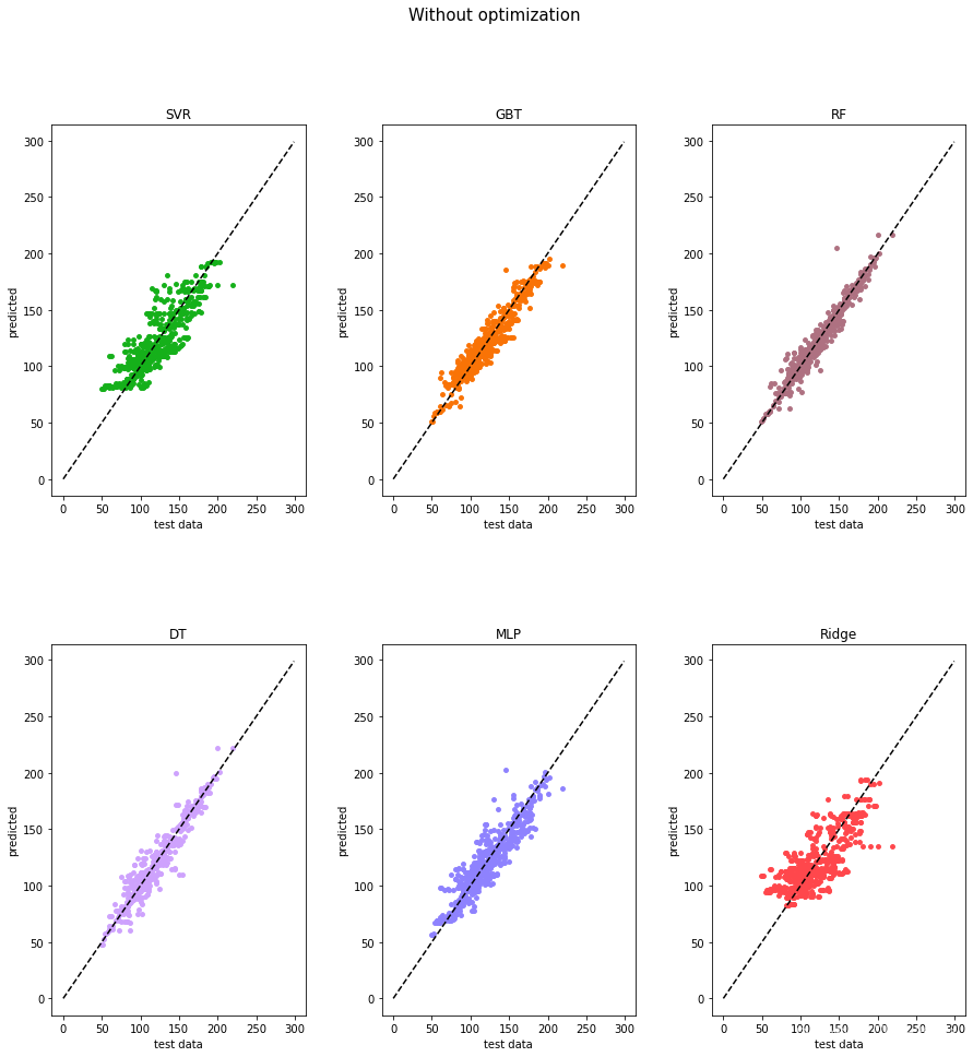
Figure 4: Scatter plots comparing predicted vs. actual hardness values for all six models without optimization. Closer alignment to the diagonal line indicates better predictions.

# 5-fold cross-validation R2
def cross_val_R2(model,X,y,test_size=0.25):
    from sklearn.model_selection import cross_val_score,ShuffleSplit
    scores_model=cross_val_score(estimator=model,
                                 X=X,
                                 y=y,
                                 cv=ShuffleSplit(n_splits=100,test_size=test_size),
                                scoring='r2') # ShuffleSplit shuffles data
    return np.mean(scores_model)

With Hyperparameter Optimization

# SVR parameter tuning
from sklearn.model_selection import GridSearchCV
from sklearn.svm import SVR
svr=SVR()

# Parameter tuning
grid_svr={'kernel':('rbf','linear',),'gamma':[0.5,1,2,4]}
gs_svr=GridSearchCV(estimator=svr,
                   param_grid=grid_svr,
                   cv=10,
                   n_jobs=-1)
gs_svr.fit(X_train,y_train.ravel())
print(gs_svr.best_params_)

# Prediction
best_svr=gs_svr.best_estimator_
best_svr.fit(X_train,y_train.ravel())
y_svr_pred_best=best_svr.predict(X_test)

{'gamma': 4, 'kernel': 'rbf'}

# GBT parameter tuning
gbt=GradientBoostingRegressor(random_state=0)

# Parameter tuning
grid_gbt={'learning_rate':[0.001,0.01,0.1,1],
         'max_depth':np.arange(7,21,7),
        'criterion':('friedman_mse','squared_error'),
         'n_estimators':[100,150,200,250]}
gs_gbt=GridSearchCV(estimator=gbt,
                   param_grid=grid_gbt,
                   cv=10,
                   n_jobs=-1)
gs_gbt.fit(X_train,y_train.ravel())
print(gs_gbt.best_params_)

# Prediction
best_gbt=gs_gbt.best_estimator_
best_gbt.fit(X_train,y_train.ravel())
y_gbt_pred_best=best_gbt.predict(X_test)

{'criterion': 'squarederror', 'learningrate': 0.1, 'maxdepth': 7, 'nestimators': 100}

# RF parameter tuning
rf=RandomForestRegressor(random_state=0)

grid_rf={'n_estimators':[70,140,210,280,350],
        'criterion':('squared_error','absolute_error'),
        'max_depth':[10,15,20,25,35,40,50],
        'min_samples_leaf':[2,4,6,8,10,12]}
gs_rf=GridSearchCV(estimator=rf,
                   param_grid=grid_rf,
                   cv=10,
                  n_jobs=-1,
                  error_score='raise')
gs_rf.fit(X_train,y_train.ravel())
print(gs_rf.best_params_)

# Prediction
best_rf=gs_rf.best_estimator_
best_rf.fit(X_train,y_train.ravel())
y_rf_pred_best=best_rf.predict(X_test)

{'criterion': 'squarederror', 'maxdepth': 15, 'minsamplesleaf': 2, 'n_estimators': 210}

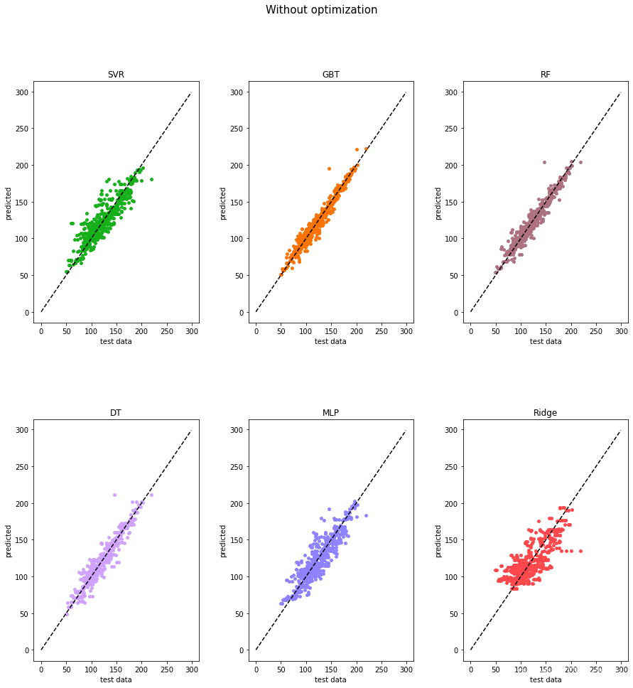
Figure 5: Scatter plots after hyperparameter optimization showing significantly improved predictions for all models. The optimized models show tighter clustering around the perfect prediction line.

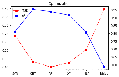
Figure 6: Comparison of MSE and R² scores after optimization. All models show substantial improvement, with GBT achieving the best overall performance.

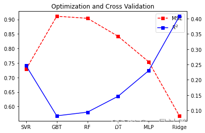
Figure 7: Cross-validation results after hyperparameter optimization, confirming the robustness of the improved models.

Summary

This study demonstrates the application of machine learning for designing aluminum alloys with enhanced hardness properties:

1. Data Preprocessing: Applied LOF (Local Outlier Factor) for anomaly detection, removing approximately 5.5% outliers from the dataset

1. Feature Selection: Combined filter and wrapper methods to identify most relevant features:

• Filter method: Removed features with low correlation (|r| < 0.45) to hardness
• RFE: Selected top 14 features for optimal performance
• Key finding: Processing time and temperature show strong correlation with hardness

1. Model Comparison: Evaluated six regression models (SVR, GBT, RF, DT, MLP, Ridge):

• Without optimization: Random Forest and Gradient Boosting showed promising results
• With optimization: Significant improvement in all models, with optimized GBT achieving best performance

1. Hyperparameter Optimization: Used GridSearchCV with 10-fold cross-validation:

• SVR: RBF kernel with gamma=4 performed best
• GBT: Optimal parameters - learningrate=0.1, maxdepth=7, n_estimators=100
• RF: Optimal parameters - nestimators=210, maxdepth=15

1. Validation: Employed cross-validation and separate test set evaluation to ensure generalization

This machine learning framework provides a cost-effective approach for alloy design, significantly reducing experimental trials and accelerating the development of high-performance aluminum alloys.