Machine Learning Support Vector Machines

This post covers Support Vector Machines (SVMs), one of the most powerful supervised learning algorithms, including the math behind large margin classification and kernel methods.

Support Vector Machines

From Logistic Regression to SVM

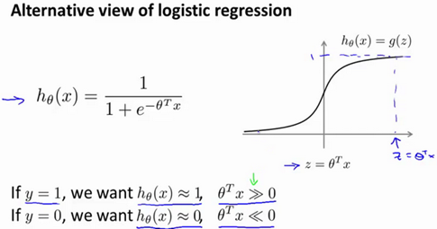
Logistic Regression Recap:

• Hypothesis: h_θ(x) = 1/(1 + e^(-θᵀx))
• Cost for single example:
• If y=1: -log(h_θ(x))
• If y=0: -log(1 - h_θ(x))

SVM Modification:

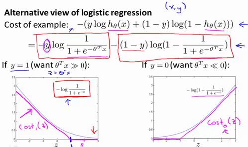
Replace smooth log curves with piecewise linear "hinge loss":

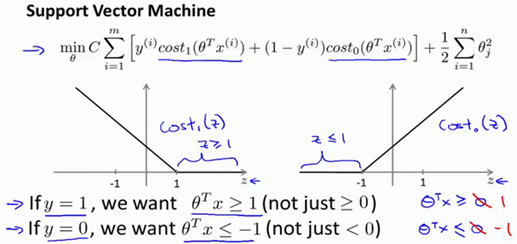
• cost₁(z): For y=1, penalizes when z < 1 (not just z < 0)
• cost₀(z): For y=0, penalizes when z > -1 (not just z > 0)

SVM Optimization Objective:

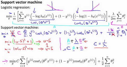
$\min\theta C \sum{i=1}^{m} [y^{(i)}\text{cost}1(\theta^T x^{(i)}) + (1-y^{(i)})\text{cost}0(\theta^T x^{(i)})] + \frac{1}{2}\sum{j=1}^{n}\thetaj^2$

Where:

• C ≈ 1/λ (larger C → lower regularization → potential overfitting)
• We removed 1/m (doesn't affect optimization)

SVM Predictions:

• If θᵀx ≥ 0: predict y = 1
• If θᵀx < 0: predict y = 0
• (No probability output, unlike logistic regression)

Large Margin Intuition

Stricter Classification Requirements:

• For y=1: Wants θᵀx ≥ 1 (not just ≥ 0)
• For y=0: Wants θᵀx ≤ -1 (not just < 0)
• Creates a "safety margin" beyond just correct classification

When C is very large:
SVM tries to make all costs₀/cost₁ terms zero, simplifying to:
$\min\theta \frac{1}{2}\sum{j=1}^{n}\theta_j^2$
Subject to:

• θᵀx⁽ⁱ⁾ ≥ 1 if y⁽ⁱ⁾ = 1
• θᵀx⁽ⁱ⁾ ≤ -1 if y⁽ⁱ⁾ = 0

Geometric Result:
SVM finds the decision boundary that:

1. Separates the classes
2. Maximizes the margin (distance to nearest points from either class)

This makes SVM a Large Margin Classifier.

C Parameter Effects:

• Large C: Small margin, low bias, high variance (may overfit to outliers)

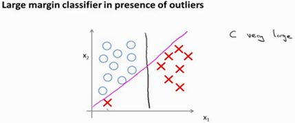
• Small C: Large margin, high bias, low variance (more robust to outliers)

Mathematics of Large Margin (Optional)

Vector Inner Product Review:

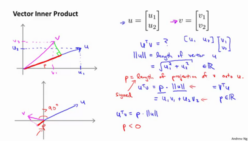
• u·v = ||u|| × ||v|| × cos(θ)
• u·v = p × ||u|| where p = signed projection of v onto u

SVM Objective in Vector Form:
$\min_\theta \frac{1}{2}||\theta||^2$

Subject to: p⁽ⁱ⁾ · ||θ|| ≥ 1 or ≤ -1

Where p⁽ⁱ⁾ = projection of x⁽ⁱ⁾ onto θ

Key Insight:

• To minimize ||θ||, SVM needs large |p⁽ⁱ⁾|
• Large projections = large margins!
• Geometric consequence: Decision boundary perpendicular to θ maximizes margins

Kernels: Non-linear Decision Boundaries

Motivation: How to efficiently create complex, non-linear boundaries?

Kernel Approach:
Instead of polynomial features, use similarity functions (kernels)

Example: Gaussian Kernel (RBF):

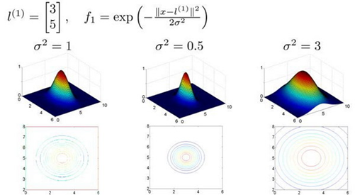
$f_i = \text{similarity}(x, l^{(i)}) = \exp\left(-\frac{||x - l^{(i)}||^2}{2\sigma^2}\right)$

Where:

• l⁽ⁱ⁾: "Landmark" points
• σ: Bandwidth parameter

Properties:

• f ≈ 1 when x ≈ l (close to landmark)
• f ≈ 0 when x far from l
• σ controls decay rate:
• Small σ: Narrow peak (high variance, low bias)
• Large σ: Wide peak (low variance, high bias)

Choosing Landmarks:
Use training examples as landmarks:

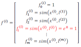
• m landmarks: l⁽¹⁾ = x⁽¹⁾, l⁽²⁾ = x⁽²⁾, ..., l⁽ᵐ⁾ = x⁽ᵐ⁾
• For each x, compute feature vector: f = [f₀, f₁, ..., f_m]ᵀ where f₀ = 1

SVM with Kernels:
$\min\theta C \sum{i=1}^{m} [y^{(i)}\text{cost}1(\theta^T f^{(i)}) + (1-y^{(i)})\text{cost}0(\theta^T f^{(i)})] + \frac{1}{2}\sum{j=1}^{m}\thetaj^2$

Predict y=1 if θᵀf ≥ 0

Kernel Trick Benefit:
Efficient computation even in infinite-dimensional feature spaces!

SVM Implementation

Don't write your own optimizer!
Use established libraries:

• liblinear (linear kernels)
• libsvm (various kernels)
• scikit-learn (Python)

Parameters to Choose:

1. C (regularization):

• Large C: Low bias, high variance
• Small C: High bias, low variance

1. Kernel choice:

• Linear kernel: k(x, l) = xᵀl
• Use when n is large, m is small
• No kernel parameters needed
• Gaussian (RBF) kernel: k(x, l) = exp(-||x-l||²/(2σ²))
• Use when n is small, m is moderate/large
• Need to choose σ²

Other Kernels (must satisfy Mercer's theorem):

• Polynomial: k(x, l) = (xᵀl + c)^d
• String kernels (for text)
• Chi-square, intersection kernels (for images)

Multi-class Classification:
Most SVM libraries have built-in one-vs-all implementation

Logistic Regression vs. SVM

Decision Guide (n = # features, m = # training examples):

Scenario	Recommended Algorithm
n >> m (e.g., n=10,000, m=10-1,000)	Logistic regression or SVM with linear kernel
n small, m intermediate (e.g., n=1-1,000, m=10-10,000)	SVM with Gaussian kernel
n small, m large (e.g., n=1-1,000, m=50,000+)	Add features, then logistic regression or linear SVM

Neural Networks:

• Generally work well for all above cases
• May be slower to train
• Optimization is non-convex (local minima)

SVM Advantages:

• Convex optimization (global optimum guaranteed)
• Less prone to local minima than neural networks
• Very effective in high-dimensional spaces

---

Key Takeaways

1. SVMs maximize the margin between classes, creating robust decision boundaries
2. C parameter trades off between:

• Fitting training data (large C)
• Maintaining large margins (small C)

1. Kernels enable non-linear decision boundaries without explicit high-dimensional feature computation
2. Gaussian kernel parameters:

• C controls regularization
• σ² controls feature width/smoothness

1. Feature scaling is critical for SVMs (especially with Gaussian kernels)
2. Don't implement from scratch - use established libraries
3. Choice between logistic regression, SVM, and neural networks depends on:

• Relative sizes of n and m
• Computational resources
• Need for interpretability

SVMs remain one of the most powerful and widely-used classification algorithms, particularly effective for medium-sized datasets with complex decision boundaries!