Machine Learning Clustering and Dimensionality Reduction

This post explores unsupervised learning techniques including K-means clustering and Principal Component Analysis (PCA) for dimensionality reduction.

K-Means Clustering

What is Clustering?

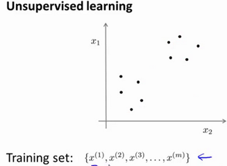
Unsupervised Learning: Finding structure in unlabeled data {x⁽¹⁾, x⁽²⁾, ..., x⁽ᵐ⁾} without y labels

Clustering: Automatically group data into cohesive clusters

Applications:

• Market segmentation (customer groups)
• Social network analysis (friend circles)
• Data center optimization (server groupings)
• Astronomical data analysis (galaxy formation)

K-Means Algorithm

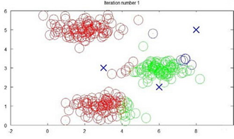
Goal: Partition data into K distinct clusters

Algorithm Steps:

1. Randomly initialize K cluster centroids μ₁, μ₂, ..., μ_K
2. Repeat until convergence:
   a. Cluster assignment: Assign each point to nearest centroid

![K-Means Iteration 1](/images/blog/2023-08-05-ml-week8-clustering-dimensionality-reduction/kmeans-iteration1.png)

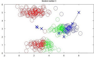
      c⁽ⁱ⁾ = index of closest centroid to x⁽ⁱ⁾
   b. Move centroids: Update each centroid to mean of assigned points

![K-Means Iteration 3](/images/blog/2023-08-05-ml-week8-clustering-dimensionality-reduction/kmeans-iteration3.png)

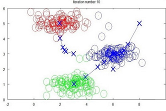
      μ_k = average of points assigned to cluster k

Detailed Steps:

Step 1 - Cluster Assignment:
For each training example x⁽ⁱ⁾:
$c^{(i)} = \arg\mink ||x^{(i)} - \muk||^2$

Step 2 - Move Centroids:
For each cluster k:
$\muk = \frac{1}{|Ck|} \sum{i \in Ck} x^{(i)}$

where C_k = set of examples assigned to cluster k

Convergence: Centroids no longer move (or move very little)

Optimization Objective

K-means minimizes the distortion function:
$J(c, \mu) = \frac{1}{m}\sum{i=1}^{m}||x^{(i)} - \mu{c^{(i)}}||^2$

• Cluster assignment step: Minimizes J holding μ fixed
• Move centroids step: Minimizes J holding c fixed
• J should never increase during iterations

Debugging: If J increases, there's a bug in your implementation!

Random Initialization

Recommended Method:

1. Choose K < m
2. Randomly select K training examples
3. Set μ₁, ..., μ_K equal to these K examples

Problem: Local Optima

K-means can get stuck in local optima depending on initialization

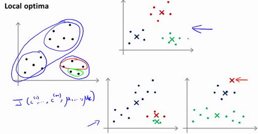
Solution: Multiple Random Initializations:

best_cost = infinity
for i in range(50 to 1000):
    # Randomly initialize centroids
    # Run K-means
    # Compute cost J
    if J < best_cost:
        best_cost = J
        best_clusters = current_clusters

Works well for small K (2-10), less benefit for larger K

Choosing K

Elbow Method:

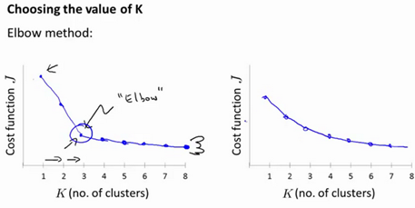
1. Run K-means for different K values
2. Plot cost J vs. K
3. Look for "elbow" where J starts decreasing slowly

Often ambiguous! No clear elbow in many datasets.

Better Approach: Choose K based on downstream purpose

• T-shirt sizes: K=3 (S, M, L) vs. K=5 (XS, S, M, L, XL)

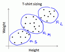
• Evaluate which K better serves business goals

Principal Component Analysis (PCA)

Motivation for Dimensionality Reduction

1. Data Compression

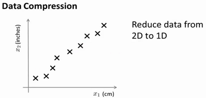
Redundant Features Example:

• Length in cm and length in inches → 1D representation
• 1000 features → 100 features (90% compression!)

Benefits:

• Saves disk space/memory
• Speeds up learning algorithms

2. Data Visualization

Cannot visualize > 3 dimensions directly

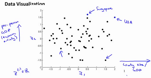
Example: Country data with 50 features (GDP, life expectancy, etc.)

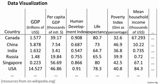
• Reduce to 2D or 3D
• Plot and discover patterns (rich vs. poor countries)

Challenge: New features may lack interpretable meaning

PCA Problem Formulation

Goal: Find lower-dimensional surface that minimizes projection error

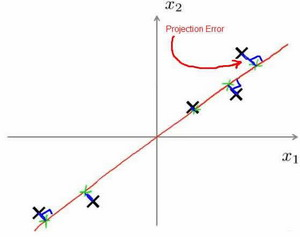
From n dimensions to k dimensions:
Find k vectors u⁽¹⁾, ..., u⁽ᵏ⁾ onto which to project data such that projection error is minimized

PCA vs. Linear Regression:

PCA	Linear Regression
Minimizes orthogonal distance to surface	Minimizes vertical distance to line
All features treated equally	Distinguishes x (input) and y (output)
Unsupervised	Supervised

PCA is NOT linear regression!

PCA Algorithm

Preprocessing: Feature scaling/mean normalization
$xj = \frac{xj - \muj}{sj}$

Steps:

1. Compute covariance matrix:
$\Sigma = \frac{1}{m}\sum_{i=1}^{m}(x^{(i)})(x^{(i)})^T$
(Σ is n×n matrix)

2. Compute eigenvectors using Singular Value Decomposition:

[U, S, V] = svd(Sigma);

• U is n×n matrix with eigenvectors as columns
• Take first k columns of U: U_reduce (n×k matrix)

3. Compute new features:
$z^{(i)} = U_{reduce}^T x^{(i)}$

• x⁽ⁱ⁾ is n×1, U_reduce^T is k×n
• z⁽ⁱ⁾ is k×1 (reduced dimension)

Choosing k (Number of Principal Components)

Goal: Retain most variance while reducing dimensions

Variance Retention: Typically choose k such that 95-99% variance is retained

Formula:
$\frac{\sum{i=1}^{k}S{ii}}{\sum{i=1}^{n}S{ii}} \geq 0.99$

where S is the diagonal matrix from SVD

Algorithm:

for k in range(1, n+1):
    variance_retained = sum(S[0:k,0:k]) / sum(S[:,:])
    if variance_retained >= 0.99:
        return k

No need to loop! Can compute directly from S matrix

Reconstruction from Compressed Representation

Approximate reconstruction:
$x{approx} = U{reduce} \cdot z$

• z is k×1 compressed representation
• x_approx is n×1 approximate original
• Lies on k-dimensional subspace

Practical Advice for PCA

Correct Usage:

1. Run PCA only on training set
2. Get U_reduce from training set
3. Apply same transformation to CV and test sets

Common Mistakes:

❌ Using PCA to prevent overfitting

• PCA doesn't use labels y
• May throw away valuable information
• ✅ Use regularization instead

❌ Defaulting to PCA in every project

• Try full features first
• Only use PCA if:
• Training is too slow
• Memory issues
• Visualization needed

When NOT to use PCA:

• If original features work well, don't add complexity
• PCA loses information (even if 99% retained, 1% may be critical)

---

Clustering Evaluation Metrics

Homogeneity: Cluster purity (like precision)
Completeness: All same-class items in same cluster (like recall)
V-measure: Harmonic mean of homogeneity and completeness
Silhouette Coefficient: Measures how similar object is to its cluster vs. other clusters

$s(i) = \frac{b(i) - a(i)}{\max\{a(i), b(i)\}}$

Where:

• a(i): Avg distance to points in same cluster
• b(i): Avg distance to points in nearest other cluster
• s(i) ∈ [-1, 1], higher is better

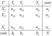
Adjusted Rand Index (ARI): Similarity between two clusterings, adjusted for chance

Key Takeaways

1. K-means finds compact clusters by iteratively assigning points and moving centroids
2. Always run multiple random initializations to avoid poor local optima
3. Choose K based on application needs, not just elbow method
4. PCA reduces dimensions while preserving variance
5. PCA is for compression and visualization, NOT preventing overfitting
6. Always try original features first before applying PCA
7. Feature scaling is critical for both K-means and PCA
8. PCA parameters learned on training set only, then applied to CV/test sets

These unsupervised learning techniques are fundamental tools for exploratory data analysis and preprocessing in machine learning pipelines!