Large Scale Machine Learning: Efficient Training for Big Data

This post covers techniques for training machine learning models efficiently on massive datasets, including stochastic gradient descent and online learning.

Learning with Large Datasets

The Big Data Challenge

Why Large Datasets?

• More data often leads to better performance
• Especially for low-bias (complex) algorithms

Computational Problem:

• Batch gradient descent with m = 100,000,000
• Each iteration sums over 100 million examples!
• Computational cost becomes prohibitive

Do You Really Need All That Data?

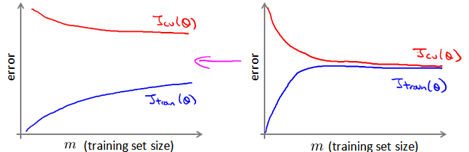
Learning Curve Sanity Check:

1. Train on small subset (e.g., m = 1,000)
2. Plot learning curves (training and CV error vs. m)
3. Analyze the curves:

• High variance: More data will help
• High bias: More data won't help much (fix model first!)

Decision:

• If curves show high variance → Proceed with large dataset
• If curves show high bias → Add features or complexity before scaling

Stochastic Gradient Descent (SGD)

The Problem with Batch Gradient Descent

Batch GD Cost Function:
$J(\theta) = \frac{1}{2m}\sum{i=1}^{m}(h\theta(x^{(i)}) - y^{(i)})^2$

Update Rule:
$\thetaj := \thetaj - \alpha \frac{1}{m}\sum{i=1}^{m}(h\theta(x^{(i)}) - y^{(i)})x_j^{(i)}$

Problem: Sum over ALL m examples in every iteration

Stochastic Gradient Descent

Key Idea: Update parameters using ONE example at a time

Cost for Single Example:
$\text{cost}(\theta, (x^{(i)}, y^{(i)})) = \frac{1}{2}(h_\theta(x^{(i)}) - y^{(i)})^2$

Algorithm:

1. Randomly shuffle training set
2. Repeat (1-10 times) {
     for i = 1 to m {
       θⱼ := θⱼ - α(h_θ(x⁽ⁱ⁾) - y⁽ⁱ⁾)xⱼ⁽ⁱ⁾  (for j=0 to n)
     }
   }

Characteristics:

• Speed: Much faster than batch GD
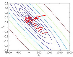
• Path: "Drunken walk" toward minimum
• Convergence: Wanders near minimum, doesn't converge precisely
• Result: Good enough for most applications

Comparison:

• Batch GD: Smooth path to minimum
• SGD: Noisy path, faster progress

Mini-Batch Gradient Descent

Compromise: Use b examples per update (2 ≤ b ≤ 100)

Algorithm:

Repeat {
  for i = 1, b+1, 2b+1, ... {
    θⱼ := θⱼ - α(1/b)Σₖ₌ᵢⁱ⁺ᵇ⁻¹(h_θ(x⁽ᵏ⁾) - y⁽ᵏ⁾)xⱼ⁽ᵏ⁾
  }
}

Advantages:

• Better than SGD for vectorized implementations
• Can use parallel hardware efficiently
• More stable than SGD, faster than batch GD

Typical Choices: b = 10, 100

Checking for Convergence

Challenge: How to know if SGD is working?

Monitoring Cost:

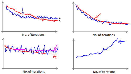
• Compute cost(θ, (x⁽ⁱ⁾, y⁽ⁱ⁾)) before updating θ
• Every 1000 iterations, plot average cost of last 1000 examples

Interpreting Plots:

1. Decreasing curve: Learning is working

• Use more averaging (5000 examples) for smoother curve

1. Flat curve: May need smaller learning rate α

1. Increasing curve: Use smaller α

Learning Rate Strategies:

Constant α:

• Simple, often works well
• May oscillate near minimum

Decreasing α:
$\alpha = \frac{\text{const1}}{\text{iterationNumber} + \text{const2}}$

• Converges closer to minimum
• Need to tune const1, const2
• Usually not worth the effort

Online Learning

Continuous Learning from Data Streams

Scenario: Website with continuous user traffic

Example - Shipping Service:

• User queries: origin, destination
• Features x: origin, destination, price
• Label y: Did user choose our service? (1/0)
• Goal: Learn p(y=1|x;θ) to optimize pricing

Online Learning Algorithm:

Repeat forever {
  Get (x,y) from user
  Update: θⱼ := θⱼ - α(h_θ(x) - y)xⱼ  (for all j)
  Discard (x,y)
}

Key Characteristics:

• No stored dataset: Process each example once
• Adapts to changes: User preferences evolve over time
• Scales infinitely: Can handle unlimited data
• Memory efficient: No need to store historical data

Applications

1. Product Search

• User searches for phones
• Show 10 phone options
• y = which phones user clicks
• Learn p(click) for better ranking

2. Package Delivery

• Offer 3 shipping options
• User selects 2
• Generates 3 training examples (2 positive, 1 negative)
• Update model immediately

3. Personalized News

• Features: article keywords, user history
• y: Did user click?
• Learn personalized click-through rate (CTR)

Advantages:

• Adapts to changing trends
• No storage limits
• Always up-to-date
• Can handle massive scale (millions of users)

vs. Batch Learning:

• Batch: Fixed dataset, retrain periodically
• Online: Continuous updates, never stops learning

Map-Reduce and Data Parallelism

Scaling Beyond Single Machines

When Online/SGD Isn't Enough:
Some algorithms need batch processing but datasets are huge

Map-Reduce Concept:
Split computation across multiple machines/cores

Example - Batch GD with m = 400:
Split into 4 machines, each with 100 examples:

Machine 1: temp₁ = Σᵢ₌₁¹⁰⁰(h_θ(x⁽ⁱ⁾) - y⁽ⁱ⁾)x⁽ⁱ⁾
Machine 2: temp₂ = Σᵢ₌₁₀₁²⁰⁰(h_θ(x⁽ⁱ⁾) - y⁽ⁱ⁾)x⁽ⁱ⁾
Machine 3: temp₃ = Σᵢ₌₂₀₁³⁰⁰(h_θ(x⁽ⁱ⁾) - y⁽ⁱ⁾)x⁽ⁱ⁾
Machine 4: temp₄ = Σᵢ₌₃₀₁⁴⁰⁰(h_θ(x⁽ⁱ⁾) - y⁽ⁱ⁾)x⁽ⁱ⁾

Master: Combine results
θⱼ := θⱼ - α(1/400)(temp₁ + temp₂ + temp₃ + temp₄)

Applicable Algorithms:

• Any algorithm with summation over training set
• Linear regression, logistic regression, neural networks
• Can use multi-core on single machine OR cluster

Framework: Hadoop, Spark for distributed computing

Key Insight: Design algorithms as summations when possible for easy parallelization!

---

Strategy Summary

Small Dataset (m < 10,000):

• Use regular batch gradient descent
• Consider normal equation if features not too many

Medium Dataset (10,000 < m < 1,000,000):

• Try mini-batch GD (b = 10-100)
• Or SGD with learning curves monitoring

Large Dataset (m > 1,000,000):

• Stochastic Gradient Descent
• Very fast
• Good enough solution
• Easy to implement

• Mini-Batch GD
• Better for vectorization
• Can leverage parallel hardware

• Map-Reduce
• When need batch GD on huge dataset
• Have multiple machines/cores available
• Algorithm can be expressed as summation

Continuous Data Stream:

• Online Learning
• Infinite scalability
• Adapts to changes
• No storage needed

Key Takeaways

1. Check learning curves before committing to huge dataset
2. SGD is workhorse for large-scale learning

• 10-100× faster than batch GD
• "Good enough" solutions for most applications

1. Mini-batch balances speed and stability
2. Monitor convergence with running average of cost
3. Online learning for continuous data streams

• Adapts to changing distributions
• Never stops learning

1. Map-Reduce parallelizes batch algorithms

• Use when batch processing necessary
• Leverage multiple cores/machines

Golden Rule: "It's not who has the best algorithm that wins, it's who has the most data" - but only if you can process it efficiently!

These techniques are fundamental to modern large-scale machine learning systems powering web services, recommendation engines, and real-time applications.